#30DayMapChallenge 2020

2020-11-01

Intro

Last year I got drawn into the #30DayMapChallenge and made it to day 19. I was pretty disorganized, didn’t timebox my days, and had a couple double-map days. I’m not sure how much better this year will go, but I’m going to try and keep this page updated with the maps and methods throughout the month.

30 Day Map Challenge Categories

Day 1: Points

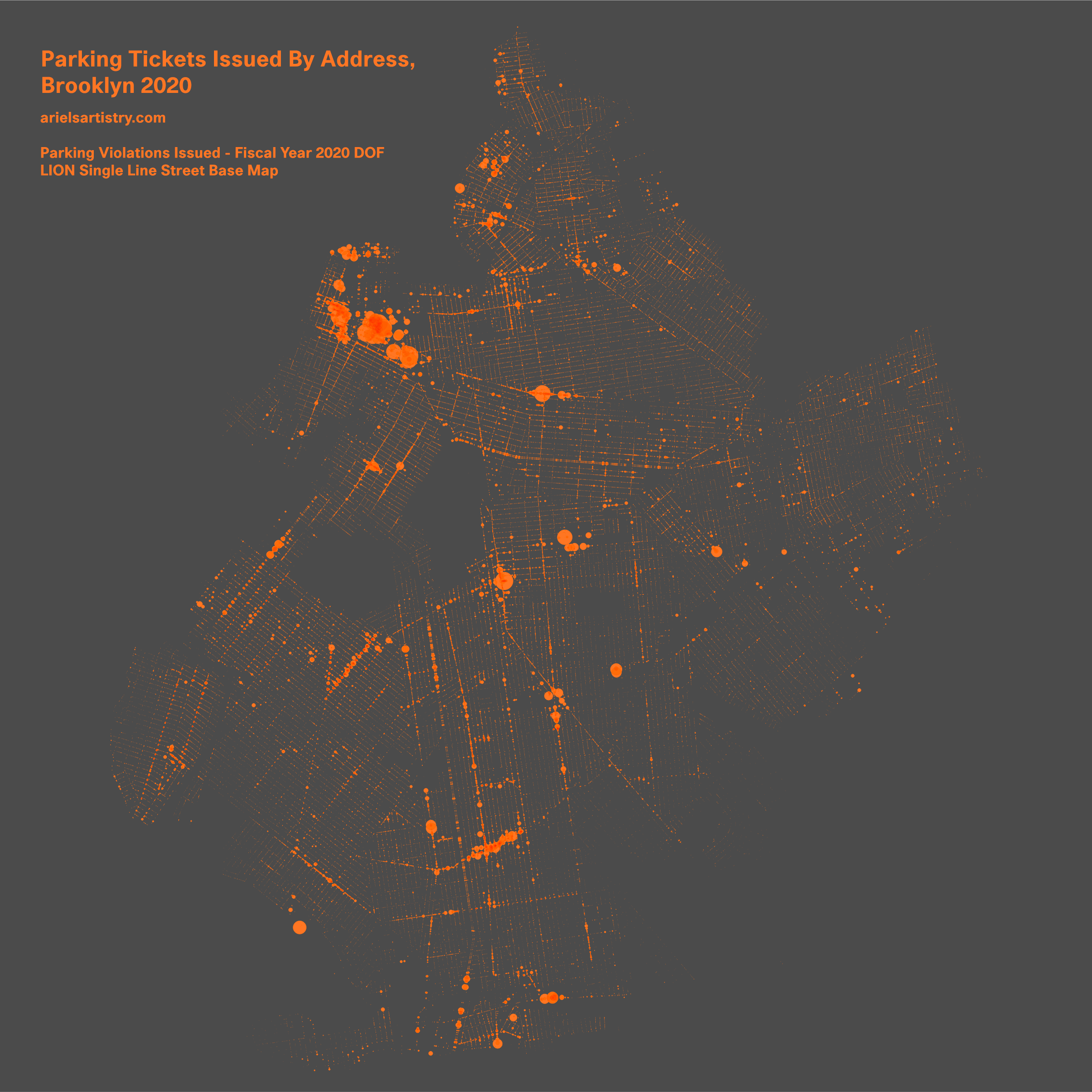Dot density/proportional symbol map recording parking violations in Brooklyn.

Data Sources

Tools

QGIS
PostgreSQL/PostGIS
Photoshop

What a start! Wouldn’t be a challenge without diving into some data. I love a good dot density map, many of which have been popping up since the challenge started. As with last year, it is tough not to be inspired by the content posted from those in time zones ahead.

For today’s map, I started surfing the NYC open data portal by most recent datasets which is where I found Parking Violations Issued - Fiscal Year 2020, though I would come to find this data contains way more than that. It comprises 43 columns and 12.5 million rows, with parking violations going back way further than 2020. One thing it is lacking though, is any sort of geocoded locations. Instead we’re given “House Number”, “Street” and “StreetCode1”, “StreetCode2”, “StreetCode3”. Along with some other geo-identifying columns.

Note not all results shown for each query.

First I loaded it into Postgresql.

COPY parking 
FROM 'Parking_Violations_Issued_-_Fiscal_Year_2020.csv'
DELIMITER ','
CSV header;

SELECT count(*) from parking;
> 12,495,734

And running some fun fact queries, like which makes have the most tickets.

SELECT vehiclemake, count(*) FROM parking GROUP BY vehiclemake ORDER BY count(*) DESC;

vechiclemake, count
TOYOT    1395273
HONDA    1343265
FORD    1328063
NISSA    1119587
CHEVR    711464
FRUEH    530846
ME/BE    530473
JEEP    490977
BMW        488545
DODGE    462646
HYUND    357747
LEXUS    293752
ACURA    247954
INTER    231149
INFIN    230237

And then look a look at some rows related to location

SELECT vehiclemake, streetcode1, violationlocation, housenumber, streetname FROM parking LIMIT 5;

vehiclemake, streetcode1, violationlocation, housenumber, streetname
TOYOT    57310    52    3604    PAUL AVE
DODGE    0       503    NULL     KINGS COLLEGE AVE
TOYOT    23920    52    3505    DECATUR AVE
NISSA    23920    52    3505    DECATUR AVE
FORD     0        52    18    VAN CORTLANDT AVE

After doing some Googling, it looks like “streetcode” is a reference to the LION dataset, which contains all the streets in NYC. Downloaded that dataset (which happened to be a ArcGIS File Geodatabase), loaded it into QGIS and attempted to import into my local PostgreSQL (with the PostGIS extension of course). It failed due to the geometry containing both MultiLineString and MultiCurve shapes. No problem, ran “Multipart to Singleparts” in the QGIS processing toolbox and was off on my way.

A look at the LION street data, this time informed by a handy metadata dictionary. The dictionary let me know some things like the streetcode in the lion dataset starts with the borough code. And that “FromLeft” to “ToLeft” describe the street numbers contained on that geometry (similarly there is a “FromRight” to “ToRight”).

SELECT count(*) FROM lion_single_parts;
> 229,208

SELECT "StreetCode", "Street", "FromLeft", "ToLeft" FROM lion_single_parts; 
435290    BEACH CHANNEL DRIVE    60001    61099
415990    76 STREET            69001    69099
439690    COOPER AVENUE        75001    75099
414890    71 AVENUE            75001    75099
457550    NORTH CONDUIT AVENUE90001    90099

In order to figure out how to join the streetcodes between these two datasets, I started with one example from the parking dataset and kept refining the query until I found the matching street. Lets use one of the examples above, 3604 PAUL AVE with street code 57310.

SELECT "StreetCode", "Street" FROM lion_single_parts WHERE "Street" LIKE '%PAUL AVE%';

"StreetCode", "Street"
266110    ST PAUL AVENUE    2007    2099
257310    PAUL AVENUE        3591    3599
266110    ST PAUL AVENUE    2001    2005
257310    PAUL AVENUE        3501    3589
257310    PAUL AVENUE        0        0
257310    PAUL AVENUE        0        0
257310    PAUL AVENUE        0        0
257310    PAUL AVENUE        0        0
257310    PAUL AVENUE        0        0
257310    PAUL AVENUE        0        0
257310    PAUL AVENUE        3401    3499
257310    PAUL AVENUE        3101    3399

Here we can see the code 57310 with the borough code 2 (Bronx) appended in front.

I decided I wanted to look just at Brooklyn parking violations in 2020, and made a handy table with the subset of those violations. One of the columns, “violationlocation”, included a precinct number which could be filtered on to Brooklyn precincts (between 60 and 94).

CREATE table streetcodes as
SELECT streetcode1, streetcode2, streetcode3, housenumber, streetname, vehiclecolor, summonsnumber
FROPM parking 
WHERE violationlocation >= 60 AND violationlocation <= 94 AND streetcode1 <> '0' AND streetcode2 <> '0' AND streetcode3 <> '0'
AND issuedate like '%2020%';

SELECT count(*) FROM streetcodes;
> 565153

Now let’s take a look at the number of violations per street.

SELECT streetname, st1."FromLeft", st1."ToLeft", count(*), st1.geom
FROM streetcodes, lion_single_parts as st1
WHERE '30' || streetcodes.streetcode1 = st1."StreetCode"
AND housenumber ~ E'^\\d+$'
AND (housenumber::integer between st1."FromLeft" AND "ToLeft")
GROUP BY st1.geom, st1."FromLeft", st1."ToLeft", streetname
ORDER BY count(*) desc;

It’s at this point I learn my SQL browser (Dbeaver) supports exporting tables in markdown.

streetname	FromLeft	ToLeft	count	geom
9th St	309	375	1084	LINESTRING (988049.3131903708 183074.34281355143, 988704.4266214818 182658.4445938021)
13th Ave	4701	4799	359	LINESTRING (986760.1262291372 171041.54244202375, 986598.2860214412 170836.28363227844)
38th St	1201	1299	336	LINESTRING (987605.216469273 173362.79415227473, 988216.0877982825 172877.91662925482)
13th Ave	4601	4699	329	LINESTRING (986921.8352368176 171245.3182516992, 986760.1262291372 171041.54244202375)
5th Ave	7101	7199	319	LINESTRING (978317.2496281117 169742.54238031805, 978216.5444233418 169418.05476491153)
13th Ave	4001	4099	316	LINESTRING (987892.2825829089 172471.13260993361, 987731.4988752753 172265.2964001447)
9th St	241	307	306	LINESTRING (987399.3146594912 183493.9646334797, 988049.3131903708 183074.34281355143)
38th St	1301	1399	306	LINESTRING (988216.0877982825 172877.91662925482, 988828.8882273883 172394.2554062754)
13th Ave	3901	3999	301	LINESTRING (988054.470690608 172673.61901953816, 987892.2825829089 172471.13260993361)

This makes sense, that block of 9th street is particularly busy and has a bus stops and bike lanes.

There is a problem though, I’m only going to know which stretch of street each parking violation is on. For a quick workaround I used ST_LineInterpolatePoints, using the house number as a rough proxy for distance along the street.

A bunch of fiddling later and…

the (almost) final query:

CREATE TABLE positions AS 
WITH streetcode AS (
    SELECT case 
        WHEN char_length(streetcode1) = 4 THEN '30' || streetcode1
        WHEN char_length(streetcode1) = 5 THEN '3' || streetcode1 
       END AS streetcodes1, housenumber, vehiclecolor, summonsnumber
    FROM streetcodes
    WHERE housenumber ~ E'^\\d+$'
), pos AS (
    SELECT st1.geom AS geom, st1."FromLeft", st1."ToLeft", housenumber, vehiclecolor, summonsnumber,
        CASE WHEN st1."ToLeft" - st1."FromLeft" = 0 THEN 0 ELSE
            (housenumber::float - st1."FromLeft") / (st1."ToLeft" - st1."FromLeft")
        END AS norm_dist
    FROM streetcode, lion_single_parts as st1
    WHERE streetcodes1 = st1."StreetCode"
    AND (housenumber::integer between st1."FromLeft" AND "ToLeft")
)
SELECT ST_LineInterpolatePoints(geom, norm_dist, false) AS geom, vehiclecolor, summonsnumber
FROM pos;

I then opened the newly created positions table in QGIS. This resulted in a ton of points overlapping and I couldn’t quiet figure out a good way to display them. Well why not throw in some porportional symbols then?

And finally another query - grouping by the geometry of each of those points in order to get a count of overlapping points.

SELECT geom, count(*)
FROM positions 
GROUP BY geom
ORDER BY count(*) desc;

I popped this final query into the QGIS Database Manager, threw on some styling to match the yellow of a parking violation, and there we have it. I skipped quite a few steps and directions I took while figuring this all out. If you have any questions feel free to reach out!

Day 2: Lines

Routes from subway stops to closet coffee shops, in the style of the Anthora coffee cup.

Data Sources:

MTA Subway Stations
LION Single Line Street Base Map
amenity=cafe from OpenStreetMap contributors (extracted using OverpassTurbo)
Font: Adonais

Tools:

QGIS
PostgreSQL/PostGIS/pgRouting
python in a jupyter notebook

No write up today, similar process to the pizza map.

Day 3: Polygons

Cartogram of NYC boroughs based on population.

Data Sources:

Census Population Estimate 2019

Tools:

python in a jupyter notebook
shapely, matplotlib

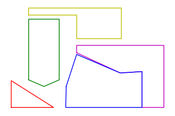
For today’s map I decided to create a cartogram of NYC using the population of each borough as the area for each polygon. After an initial sketch on paper I opened up a jupyter notebook, and started plotting away…

Some utils


import matplotlib.pyplot as plt
from shapely.geometry import Point, LineString
from shapely.wkt import loads

SHOW_POINTS = False
SHOW_POINT_LABELS = False

def plot_coord_nums(coords, color):
    count = 0
    for coord in coords:
        plt.plot(*coord, color + 'o')
        if SHOW_POINT_LABELS:
            plt.axis('on')
            plt.text(coord[0] + .1, coord[1] + .18, count, color=color)
        count += 1

def plot_shapes(shapes):
    plt.axis('off')

    for shape, color in shapes:
        if isinstance(shape, (Point, LineString)):
            plt.plot(*shape.coords.xy, color)
            if SHOW_POINTS: 
                plot_coord_nums(shape.coords, color)
        elif isinstance(shape, Polygon):
            plt.plot(*shape.exterior.coords.xy, color)
            if SHOW_POINTS: 
                plot_coord_nums(shape.exterior.coords, color)
        else:
            raise RuntimeError("Unsupported Type")

And then the shapes

print("place,        area, pop (m)")
staten = loads("POLYGON((0 0, 0 .97, .97 0, 0 0))")
print("staten.area  ", round(staten.area, 2), " 0.47")

man_left = .4
man_tip = .76
man_height = 2.2
man = loads(f"POLYGON((.4 1, .75 {man_tip}, 1.1 1, 1.1 {1 + man_height}, .4 {1 + man_height}, .4 1))")
print("man.area     ", round(man.area, 2), " 1.62")


bronx_width = 2.13
bronx = loads(f"POLYGON(({man_left} 3.35, "
              "1.5 3.35,"
              "1.5 2.5,"
              f"{man_left + bronx_width} 2.5, "
              f"{man_left + bronx_width} 3.6, "
              f"{man_left} 3.6, "
              f"{man_left} 3.35))")
print("bronx.area   ", round(bronx.area, 2), " 1.41")


brooklyn_width = bronx_width - 3
brooklyn = loads(f"POLYGON(({man_tip + .5} {man_tip}, "
                 f"1.5 1.923, "
                  "2.5 1.25,"
                  "3 1.3, "
                  "3 0, "
                 f"1.25 0, {man_tip + .5} {man_tip}))")
print("brooklyn.area", round(brooklyn.area, 2), " 2.55")


queens = loads(f"POLYGON((1.5 1.983, "
               f"1.5 1.983, "
                "2.5 1.25, "
                "3 1.3,"
                "3 0, "
                "3.5 0, "
                "3.5 2.25, "
                "1.5 2.25, "
               f"1.5 1.983))")

print("queens.area  ", round(queens.area, 2), " 2.25")


plot_shapes([(staten, 'r'), (man, 'g'),  (bronx, 'y'),  (queens, 'm'),  (brooklyn, 'b')])

place,        area, pop (m)
staten.area   0.47  0.47
man.area      1.62  1.62
bronx.area    1.41  1.41
brooklyn.area 2.55  2.55
queens.area   2.25  2.25

And for the final shape WKT’s

print("staten", staten.wkt)
print("man", man.wkt)
print("bronx", bronx.wkt)
print("brooklyn", brooklyn.wkt)
print("queens", queens.wkt)

staten POLYGON ((0 0, 0 0.97, 0.97 0, 0 0))
man POLYGON ((0.4 1, 0.75 0.76, 1.1 1, 1.1 3.2, 0.4 3.2, 0.4 1))
bronx POLYGON ((0.4 3.35, 1.5 3.35, 1.5 2.5, 2.53 2.5, 2.53 3.6, 0.4 3.6, 0.4 3.35))
brooklyn POLYGON ((1.26 0.76, 1.5 1.923, 2.5 1.25, 3 1.3, 3 0, 1.25 0, 1.26 0.76))
queens POLYGON ((1.5 1.983, 1.5 1.983, 2.5 1.25, 3 1.3, 3 0, 3.5 0, 3.5 2.25, 1.5 2.25, 1.5 1.983))

Day 4: Hexagon

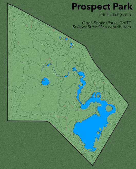Prospect Park with a simplified hexagon boundary.

Data Sources:

Open Space (Parks)
OpenStreetMap

Tools:

QGIS
Affinity Designer

Who says all these hexagon day maps need to be hexbins? This map has six(ish) sides! It’s also rotated aggressively because this is how I map Prospect Park in my mind.

First time using Affinity Designer. I like it a lot, it definitely makes more sense to be using vector image software for my maps than a raster program like Photoshop. It was easier to pick up today than any of the times I’ve ever tried to use Inkscape.

Day 5: Blue

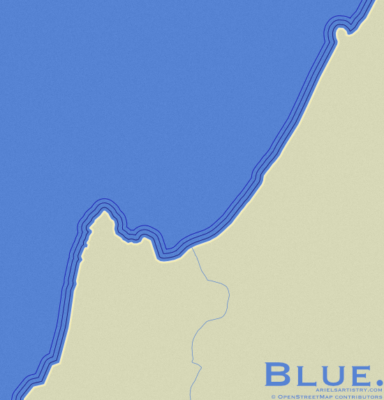Unnamed coastline in minimal style.

Data Sources:

OpenStreetMap

Tools:

QGIS
Affinity Designer

Day 6: Red

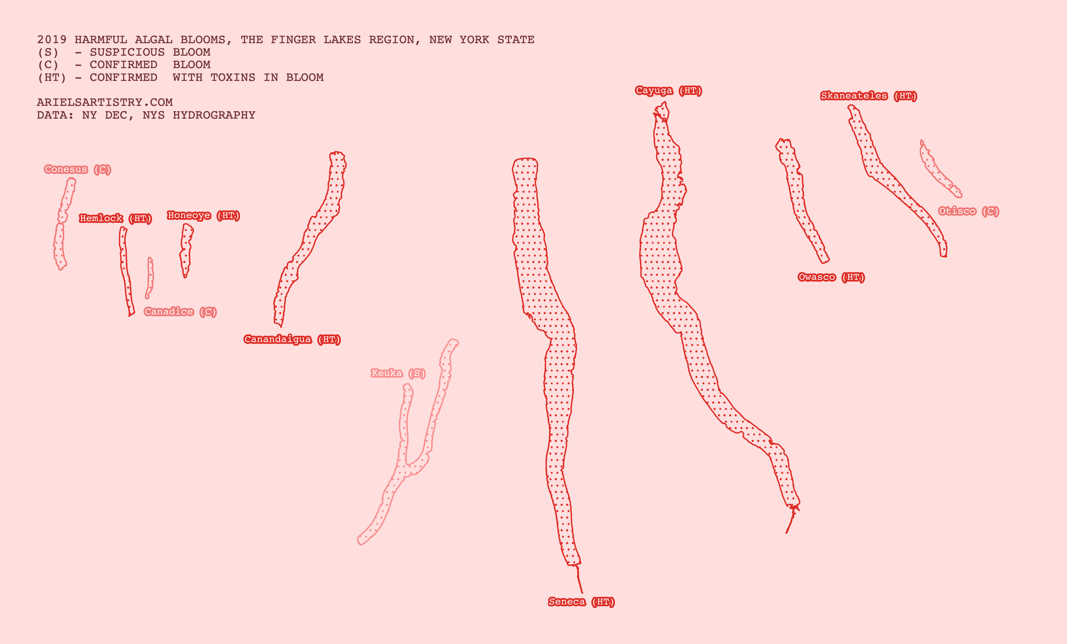2019 Algal booms status, Finger Lakes.

Data Sources:

Tools:

QGIS

Stuck with the basics today, load some data in QGIS and fiddle with the knobs.

Day 7: Green

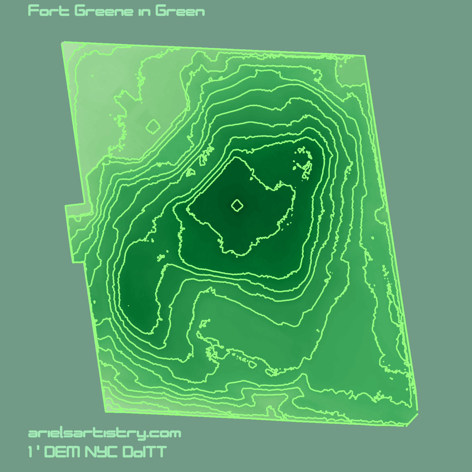Fort Greene Park in Green.

Data Sources:

Tools:

QGIS (GDAL via Processing Toolbox)

Day 8: Yellow

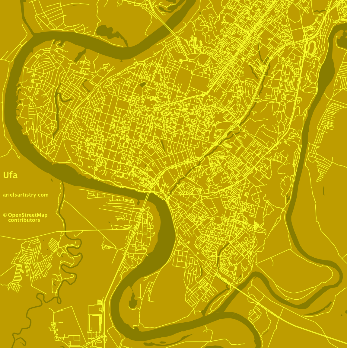Ufa in Yellow

Data Sources:

OpenStreetMap

Tools:

QGIS
Affinity Designer

Day 9: Monochrome

Monochrome Bathymetry of Lake Crescent.

Data Sources:

USGS

Tools:

QGIS
Affinity Designer

Day 10: Grid

Preview moving around NYC in interactive webmap GRID.

Data Sources:

LION Single Line Street Base Map

Tools:

Mapbox Studio, Mapbox GL JS

Controls are WASD or directional arrows. Tried to make it work on mobile but it’s going to be a bumpy ride. Use portrait mode if you do.

Enter the GRID.

Theme music - Tron Legacy - Soundtrack OST - 02 The Grid - Daft Punk

Day 11: 3D

Sunset Park Hillshade.

Data Sources:

Tools:

QGIS

Need to spend some time looking into how to make those fancy Blender maps.

Day 12: No GIS

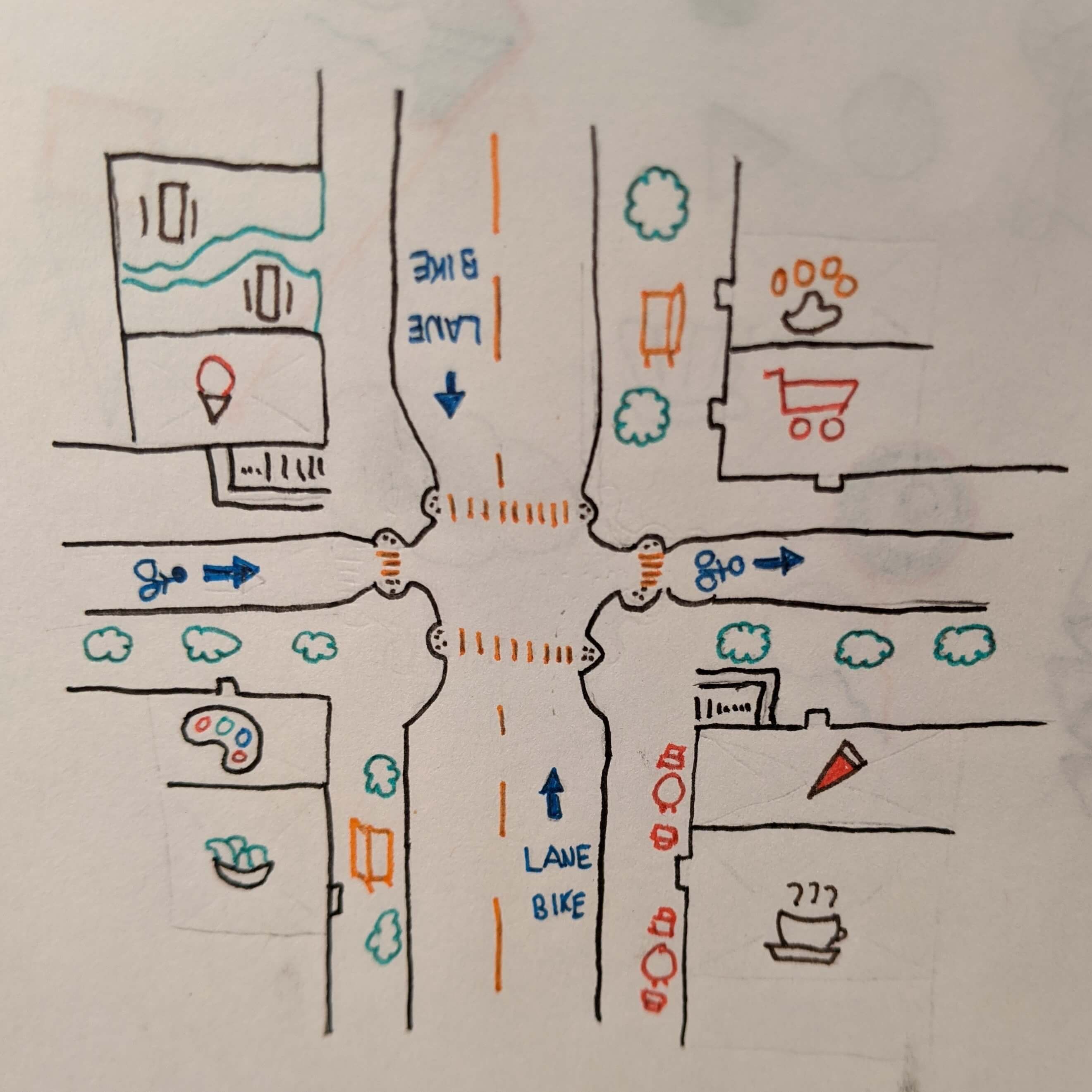Handdrawn map of fictional happy junction.

Data Sources:

Imagination

Tools:

Pencil
Paper
Stencil
Various Colored Micron Pens

Day 13: Raster

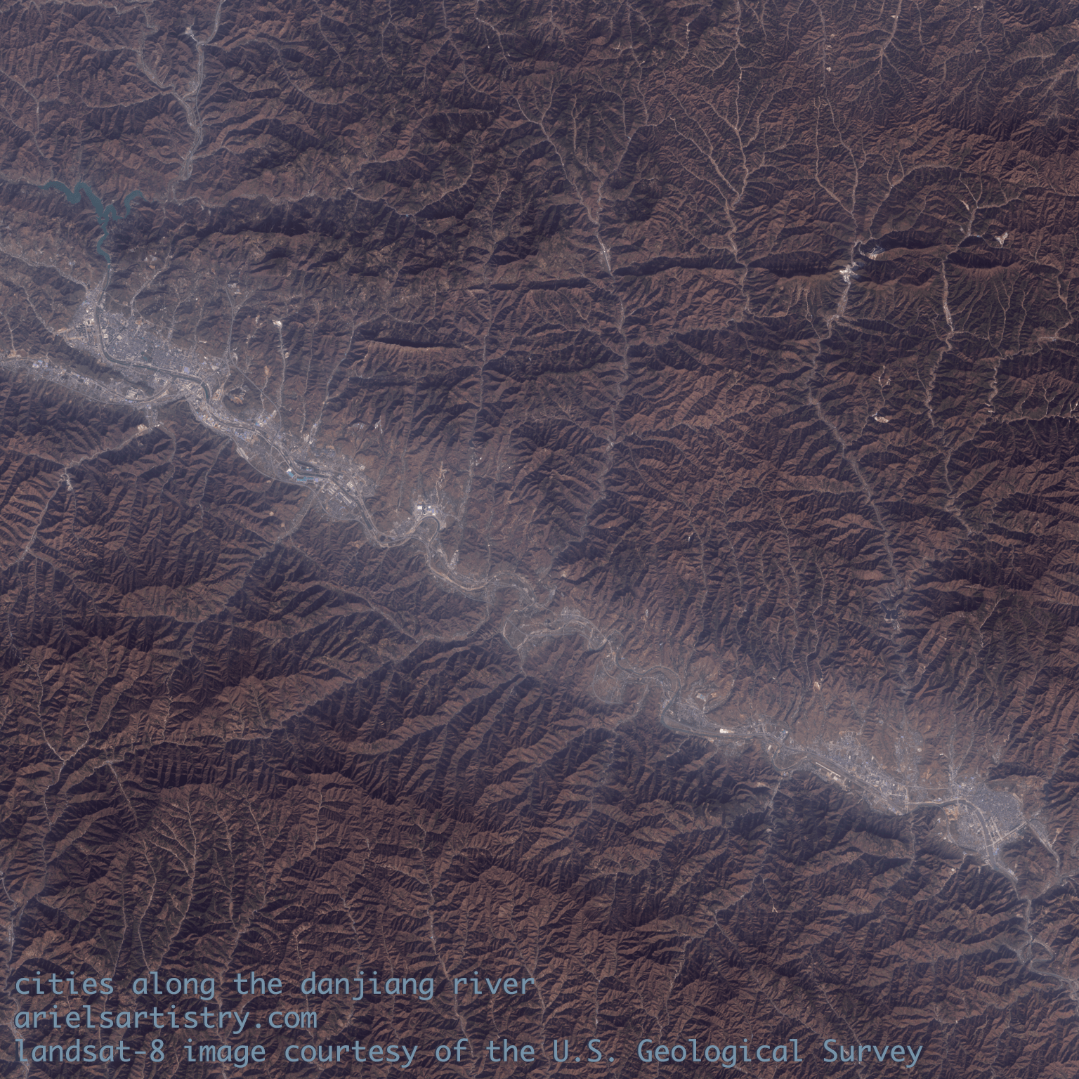Landsat-8 True Color along Danjiang River.

Data Sources:

Landsat 8 (accessed via Google Cloud)

Tools:

QGIS & GDAL (exploratory)
Photoshop

Followed this great tutorial from NASA Earth Observatory on creating true color images from Landsat 8 data. Also helped to read this article on the different bands.

Day 14: Climate Change

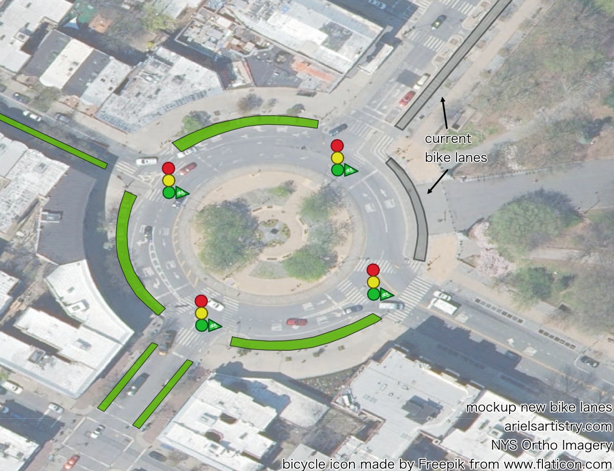Mockup new bike lanes around Bartel Pritchard Square.

Data Sources:

NYS Ortho Imagery
Bicycle Icons made by Freepik from Flaticon

Tools:

QGIS
Affinity Designer

Think about where you could use some bike lanes.

Day 15: Connections

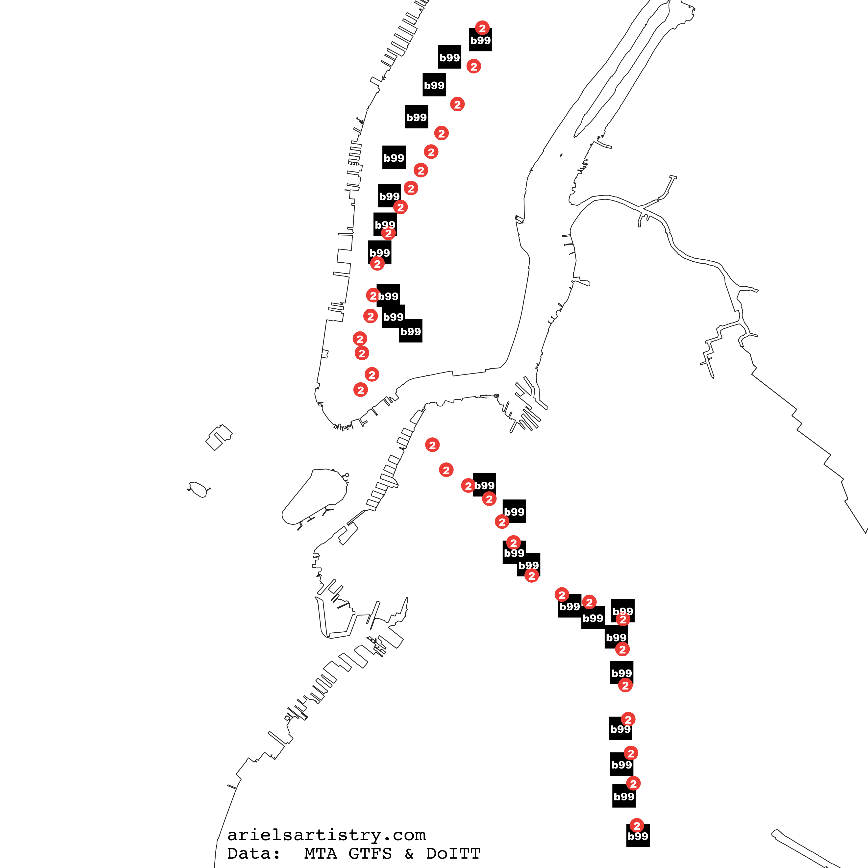Nearby stops between 2 train and B99 buses.

Data Sources:

Tools:

QGIS
PostgreSQL/PostGIS

The b99 train was added after the nightly subway shutdowns to replace the 2 train. I didn’t realize this until too far into placing the labels, otherwise I belive the A/C and b25 would have made more sense to pair. Wrote some wild queries to explore this stuff, though most I didn’t end up using. One even included HAVING.

Day 16: Islands

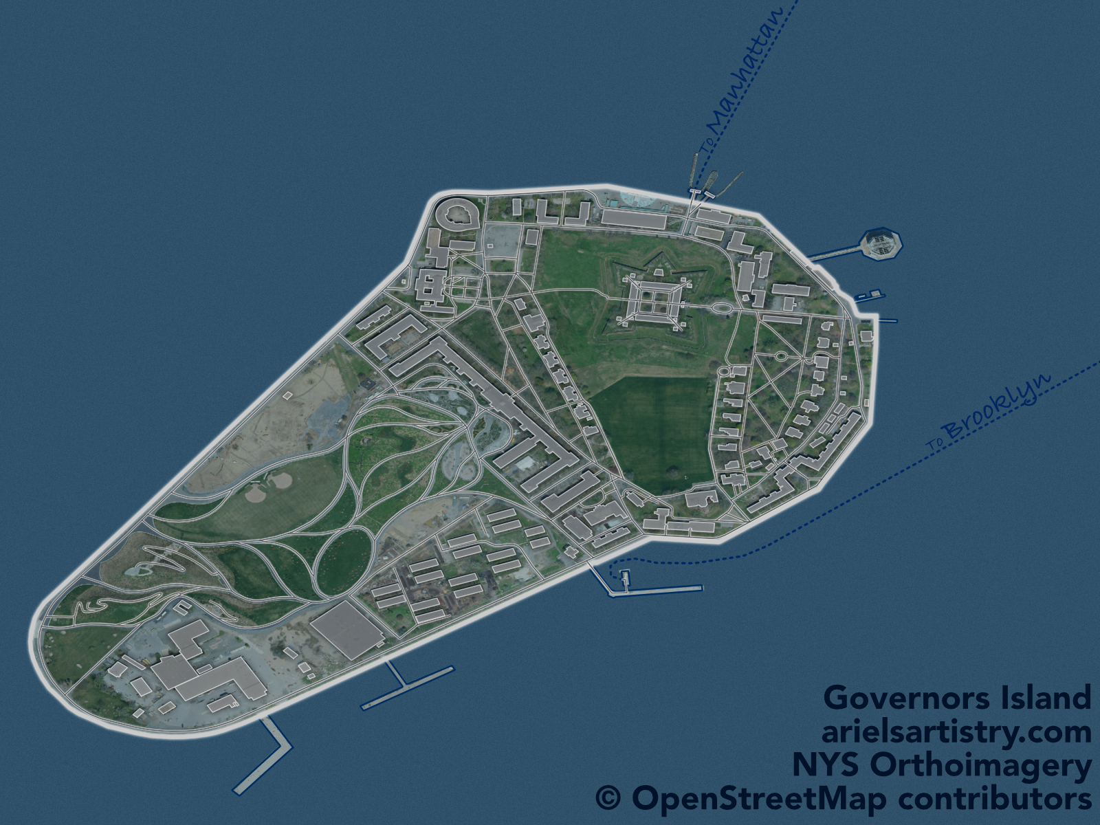Governors Island.

Data Sources:

NYS Ortho Imagery
OpenStreetMap

Tools:

QGIS
Affinity Designer

Day 17: Historical

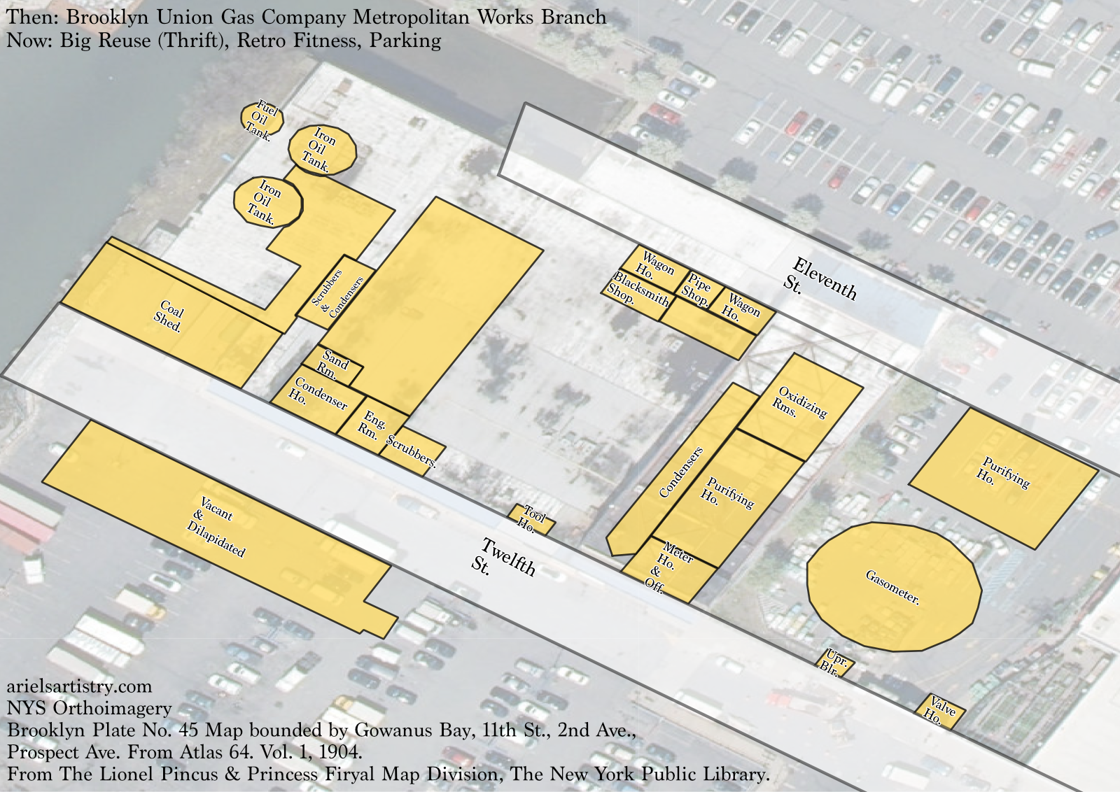Brooklyn Union Gas Company Metropolitan Works Branch, Gowanus.

Data Sources:

NYS Ortho Imagery
Brooklyn Plate No. 45 Map bounded by Gowanus Bay, 11th St., 2nd Ave., Prospect Ave.
From Atlas 64. Vol. 1, 1904. The Lionel Pincus & Princess Firyal Map Division, The New York Public Library.

Tools:

QGIS
Affinity Designer

Day 18: Landuse

A rough estimate of landuse on Manhattan Island.

Data Sources:

Tools:

QGIS
PostgreSQL/PostGIS

Shoutout to this method of stacked porportional fills using QGIS geometry generator.

The expression boils down to:

intersection($geometry, translate(bounds($geometry), 0, (PERCENT_FILL-1)*bounds_height($geometry)))

Day 19: NULL

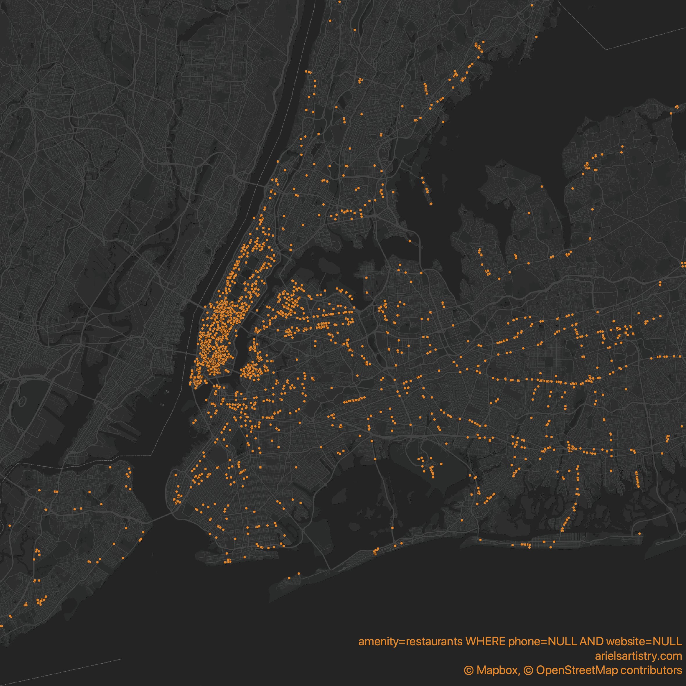Restaurants without a phone number or website on OpenStreetMap.

Data Sources:

OpenStreetMap
Mapbox (Basemap)

Tools:

QGIS
PostgreSQL/PostGIS

Day 20: Population

NYC Community Board Populations.

Data Sources:

Tools:

QGIS

Day 21: Water

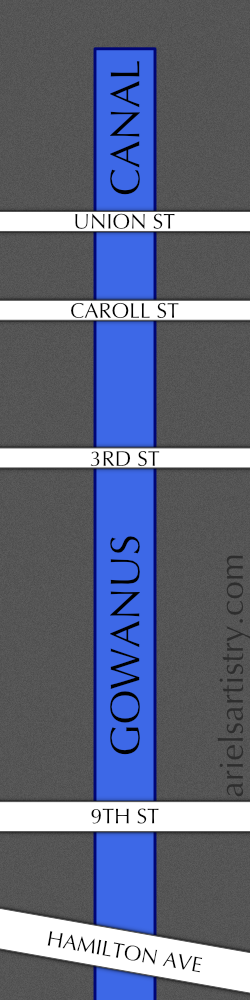Gowanus Canal Bridges.

Data Sources:

Local Knowledge
OpenStreetMap

Tools:

Affinity Designer

Day 22: Movement

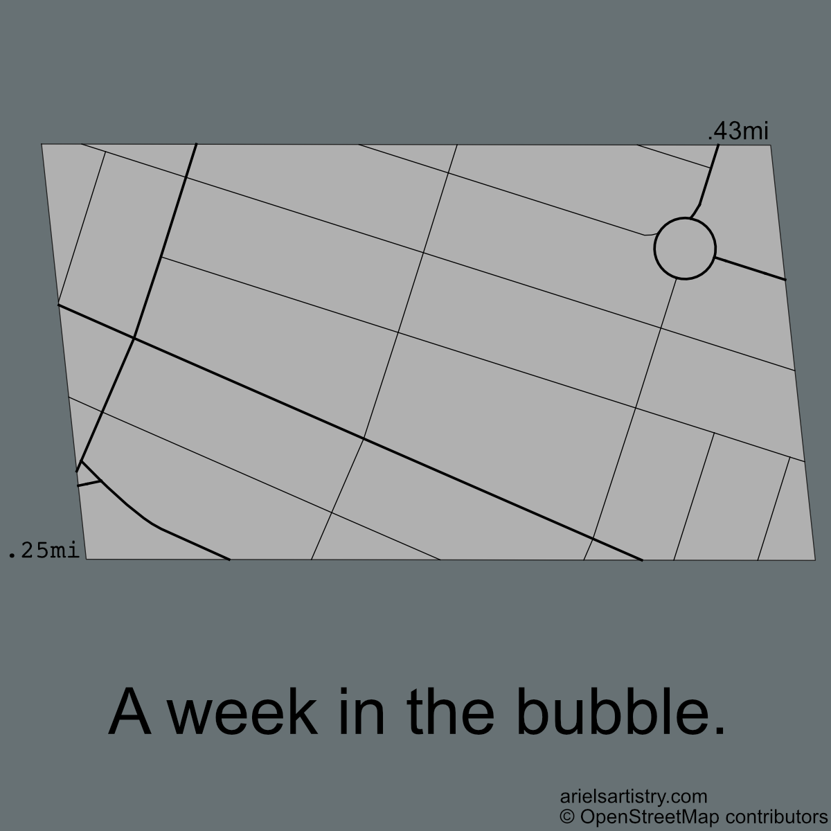The bounds of a week in my COVID bubble.

Data Sources:

OpenStreetMap

Tools:

QGIS
Affinity Designer

Day 23: Boundary

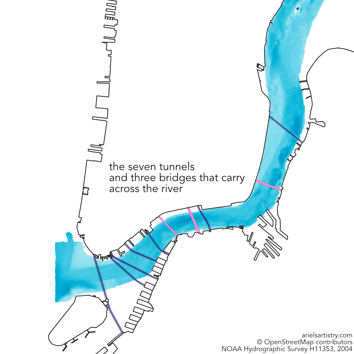Boundary between Manhattan and Brooklyn.

Data Sources:

Tools:

QGIS
Affinity Designer

Day 24: Elevation

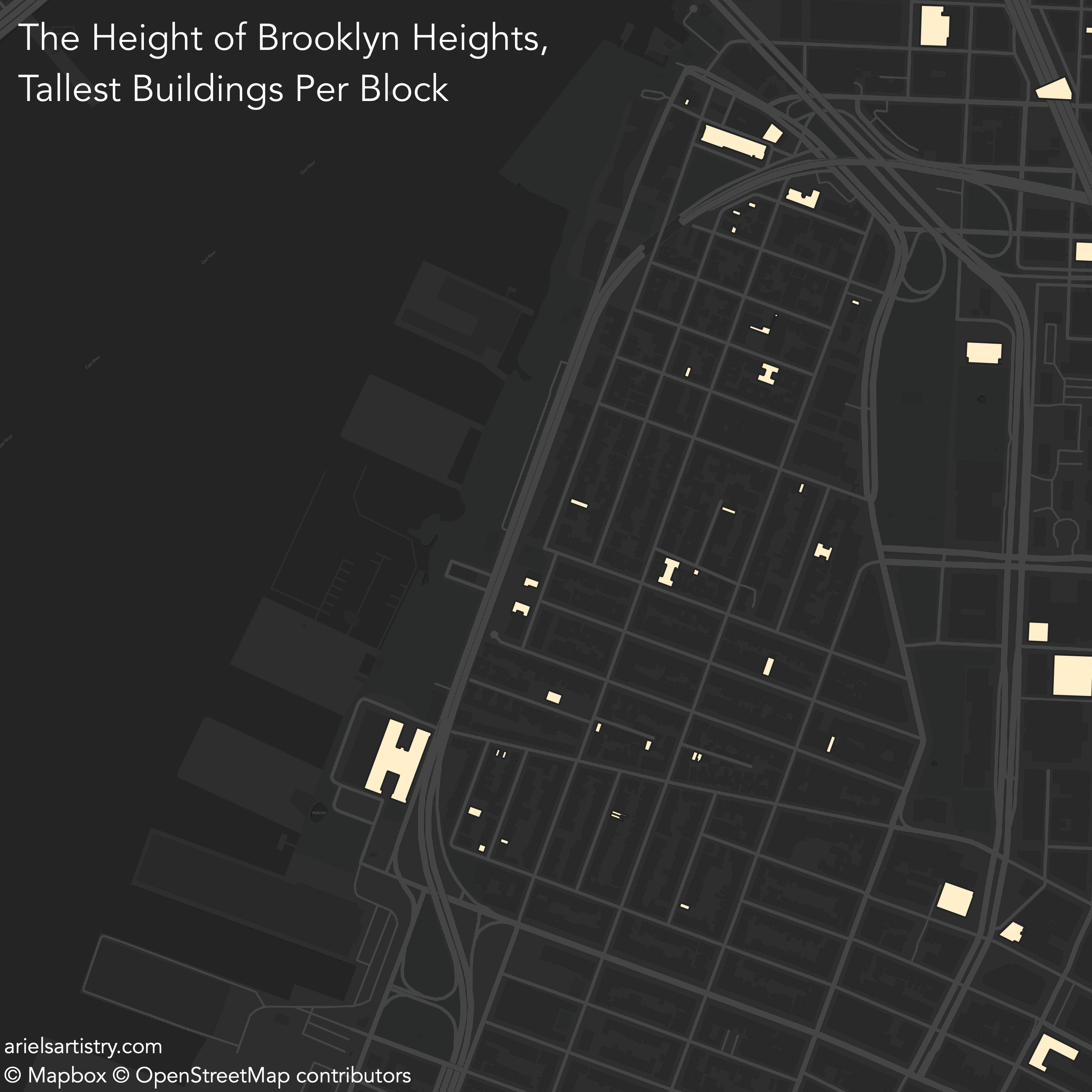Tallest buildings per block clipped on Brooklyn Heights.

Data Sources:

OpenStreetMap
Mapbox (Basemap)

Tools:

QGIS

Day 25: COVID-19

Brooklyn's "OpenStreets."

Data Sources:

NYC OpenStreets Dataset
OpenStreetMap
Mapbox (Basemap)

Tools:

QGIS

Day 26: Map With a New Tool

Attempt at adding 3D with Blender.

Data Sources:

NYC 1 Foot Integer DEM
OpenStreetMap

Tools:

QGIS
GDAL
Blender

Day 27: Big or Small Data

A small cat in a small spot.

Data Sources:

Tools:

Affinity Designer

Day 28: Non-Geographic Map

Movement In a Game of Super Bomberman R Online.

Data Sources:

Font: Nintender

Tools:

Keylogger
Super Bomberman R Online via Google Stadia

Day 29: Globe

All the places called Long Beach according to Wikipedia.

Data Sources:

Wikipedia Long Beach disambiguation

Tools:

Post-its
Sony A6000
Lightroom/Photoshop

Day 30: A Map

The genders depicted in Central Park statues.

Data Sources:

OpenStreetMap
Wikidata

Tools:

Python
QGIS

Conclusion

Well that was a fun! 30 maps in around 30 days. I can’t say I love them all, but I’m glad I put something together for each day.

Ariel Kadouri

#30DayMapChallenge 2020

Intro

Day 1: Points

Day 2: Lines

Day 3: Polygons

Day 4: Hexagon

Day 5: Blue

Day 6: Red

Day 7: Green

Day 8: Yellow

Day 9: Monochrome

Day 10: Grid

Day 11: 3D

Day 12: No GIS

Day 13: Raster

Day 14: Climate Change

Day 15: Connections

Day 16: Islands

Day 17: Historical

Day 18: Landuse

Day 19: NULL

Day 20: Population

Day 21: Water

Day 22: Movement

Day 23: Boundary

Day 24: Elevation

Day 25: COVID-19

Day 26: Map With a New Tool

Day 27: Big or Small Data

Day 28: Non-Geographic Map

Day 29: Globe

Day 30: A Map

Conclusion